Linear, Quadratic, and Regularized Discriminant Analysis
Discriminant analysis encompasses methods that can be used for both classification and dimensionality reduction. Linear discriminant analysis (LDA) is particularly popular because it is both a classifier and a dimensionality reduction technique. Quadratic discriminant analysis (QDA) is a variant of LDA that allows for non-linear separation of data. Finally, regularized discriminant analysis (RDA) is a compromise between LDA and QDA.
This post focuses mostly on LDA and explores its use as a classification and visualization technique, both in theory and in practice. Since QDA and RDA are related techniques, I shortly describe their main properties and how they can be used in R.
Linear discriminant analysis
LDA is a classification and dimensionality reduction techniques, which can be interpreted from two perspectives. The first is interpretation is probabilistic and the second, more procedure interpretation, is due to Fisher. The first interpretation is useful for understanding the assumptions of LDA. The second interpretation allows for a better understanding on how LDA performs dimensionality reduction.
The probabilistic interpretation
Each class k∈{1,…,K} is assigned a prior ˆπk such that that ∑ki=1ˆπk=1. According to Bayes’ rule, the posterior probability is
Pr(G=k|X=x)=fk(x)πk∑Kl=1fl(x)πl
where fk(x) is the density of X conditioned on k. The maximum-a-posteriori (MAP) estimator simplifies to
G(x)=argmaxkPr(G=k|X=x)=argmaxkfk(x)πk
because the denominator is identical for all classes.
LDA assumes that the density is Gaussian:
fk(x)=|2πΣk|−1/2exp(−12(x−μk)TΣ−1k(x−μk))
where Σk is the covariance matrix for the samples from class k and |.| is the determinant. LDA assumes that all classes have the same covariance matrix, i.e. Σk=Σ,∀k.
Plugging fk into the classification function, we arrive at the classification function:
G(x)=argmaxkδk(x)
where
δk(x)=xTΣ−1μk−12μTkΣ−1μk+logπk
is the discriminant function for class k. So, now that we have a classifier, how we can compute it?
To find the covariance matrix, we simply compute
ˆΣ=K∑k=11N−K∑gi=k(xi−ˆμk)(xi−ˆμk)T.
Note that the deviation from the means is divided by N−K, the degrees of freedom, to obtain an unbiased estimator.
The means of the classes, which are also called centroids, are defined by
ˆμk=1Nk∑gi=kxi.
The priors πk are set to the prevalence ratio of the class-specific observations:
ˆπk=NkN.
With this, we have defined all parameters required for the classifier.
The dimensionality reduction procedure of LDA involves the within-class variance, W=ˆΣ, and the between-class variance, B. The between-class variance indicates the deviation of centroids from the overall mean, ˆμ=∑Kk=1ˆπkˆμk, and is defined as:
B=K∑k=1ˆπk(ˆμk−ˆμ)(ˆμk−ˆμ)T.
Finding a sequence of optimal substeps involves three steps:
- Compute the K×p matrix M containing the centroids, μk, and determine the common covariance matrix W.
- Compute M∗=MW−12 using the eigen-decomposition of W.
- Compute B∗ (the between-class covariance) and its eigen-decomposition B∗=V∗DBV∗T. The columns v∗l of V∗ define the coordinates of the reduced subspace.
The l-th discriminant variable (one of the K−1 new dimensions) is determined by Zl=vTlX with vl=W−12v∗l.
The interpretation of Fisher
Fisher’s LDA optimization criterion states that the centroids of the groups should be spread out as far as possible. This amounts to finding a linear combination Z=aTX such that aT maximizes the between-class variance relative to the within-class variance.
As before, the within-class variance is W is the pooled covariance matrix, ˆΣ, which indicates the deviation of all observations from their class centroids. The between-class variance is defined according to the deviation of the centroids from the overall mean, as defined earlier. For Z, the between class variance is aTBa and the within-class variance is ATWa. Thus, LDA can be optimized through the Rayleigh quotient
maxaaTBaaTWa,
which defines an optimal mapping of X to the new space Z. Note that Z∈R1×p, that is, the observations are mapped to a single dimension. To obtain additional dimensions, we need to solve the optimization problem for a1,…,aK−1 where each successive ak is constructed to be orthogonal in W to the previous discriminant coordinates. This leads to the linear transformation G=(ZT1,ZT2,…,ZTK−1)∈Rp×q with which we can map from p to q dimension via XG. Why do we consider K−1 projections? This is because the affine subspace that is spanned by the K centroids has a rank of at most K−1.
Using Fisher’s formulation of LDA, classification involves two steps:
- Sphere the data using the common covariance matrix ˆΣ=UDUT (eigendecomposition) such that X∗=D−12UTX. In this way, the covariance of X∗ becomes the identity matrix. By eliminating the covariance between the variables in this way, it becomes much easier to separate the classes in the transformed space.
- Classify observations xi to the closest class centroid in the transformed space, taking into account the class priors πk. Here, the intuition is that an observation with equal distance to two centroids would be assigned to the class with the greater prior.
Reduced-rank LDA
LDA performs classification in a reduced subspace. When performing classification, we do not need to use all K−1 dimensions and instead can choose a smaller subspace Hl with l<K−1. When l<K−1 is used, this is called reduced-rank LDA. The motivation for reduced-rank LDA is that classification basd on a reduced number of discriminant variables can improve performance on the test set when the model is overfitted.
Complexity of the LDA model
The number of effective parameters of LDA can be derived in the following way. There are K means, ˆμk that are estimated. The covariance matrix does not require additional parameters because it is already defined by the centroids. Since we need to estimate K discriminant functions (to obtain the decision boundaries), this gives rise to K calculations involving the p elements. Additionally, we have K−1 free parameters for the K priors. Thus, the number of effective LDA parameters is Kp+(K−1).
Summary of LDA
Here, I summarize the two perspectives on LDA and give a summary of the main properties of the model.
Probabilistic view
LDA uses Bayes’ rule to determine the posterior probability that an observation x belongs to class k. Due to the normal assumption of LDA, the posterior is defined by a multivariate Gaussian whose covariance matrix is assumed to be identical for all classes. New points are classified by computing the discriminant function δk (the enumerator of the posterior probability) and returning the class k with maximal δk. The discriminant variables can be obtained through eigen-decompositions of the within-class and between-class variance.
Fisher’s view
According to Fisher, LDA can be understood as a dimensionality reduction technique where each successive transformation is orthogonal and maximizes the between-class variance relative to the within-class variance. This procedure transforms the feature space to an affine space with K−1 dimensions. After sphering the input data, new points can be classified by determining the closest centroid in the affine space under consideration of the class priors.
Properties of LDA
LDA has the following properties:
- LDA assumes that the data are Gaussian. More specifically, it assumes that all classes share the same covariance matrix.
- LDA finds linear decision boundaries in a K−1 dimensional subspace. As such, it is not suited if there are higher-order interactions between the independent variables.
- LDA is well-suited for multi-class problems but should be used with care when the class distribution is imbalanced because the priors are estimated from the observed counts. Thus, observations will rarely be classified to infrequent classes.
- Similarly to PCA, LDA can be used as a dimensionality reduction technique. Note that the transformation of LDA is inherently different to PCA because LDA is a supervised method that considers the outcomes.
The phoneme data set
To exemplify linear discriminant analysis, we will use the phoneme speech recognition data set. This data set is useful for showcasing discriminant analysis because it involves five different outcomes.
library(RCurl)
f <- getURL('https://www.datascienceblog.net/data-sets/phoneme.csv')
df <- read.csv(textConnection(f), header=T)
print(dim(df))## [1] 4509 259The data set contains samples of digitized speech for five phonemes: aa (as the vowel in dark), ao (as the first vowel in water), dcl (as in dark), iy (as the vowel in she), and sh (as in she). In total, 4509 speech frames of 32 msec were selected. For each speech frame, a log-periodogram of length 256 was computed, on whose basis we want to perform speech recognition. The 256 columns labeled x.1 to x.256 identify the speech features, while the columns g and speaker indicate the phonemes (labels) and speakers, respectively.
For evaluating models later, we will assign each sample either into the training or the test set:
#logical vector: TRUE if entry belongs to train set, FALSE else
train <- grepl("^train", df$speaker)
# remove non-feature columns
to.exclude <- c("row.names", "speaker", "g")
feature.df <- df[, !colnames(df) %in% to.exclude]
test.set <- subset(feature.df, !train)
train.set <- subset(feature.df, train)
train.responses <- subset(df, train)$g
test.responses <- subset(df, !train)$g
Fitting an LDA model in R
We can fit an LDA model in the following way:
library(MASS)
lda.model <- lda(train.set, grouping = train.responses)
Let us take a moment to investigate the relevant components of the model:
- prior contains the group priors πk and counts the corresponding group counts, Nk.
- means is the centroid matrix M∈RK×p whose components are the mean vectors, μk.
- scaling is the N×(K−1) matrix that transforms samples to the space defined by the K−1 discriminant variables.
- svd are the singular values, which indicate the ratio of between- and within-group standard deviations on the linear discriminant variables.
LDA as a visualization technique
We can transform the training data to the canonical coordinates by applying the transformation matrix on the scaled data. To obtain the same results as returned by the predict.lda function, we need to center the data around the weighted means first:
# 1. Manual transformation
# center data around weighted means & transform
means <- colSums(lda.model$prior * lda.model$means)
train.mod <- scale(train.set, center = means, scale = FALSE) %*%
             lda.model$scaling
# 2. Use the predict function to transform:
lda.prediction.train <- predict(lda.model, train.set)
all.equal(lda.prediction.train$x, train.mod)## [1] TRUEWe can use the first two discriminant variables to visualize the data:
# visualize the features in the two LDA dimensions
plot.df <- data.frame(train.mod, "Outcome" = train.responses)
library(ggplot2)
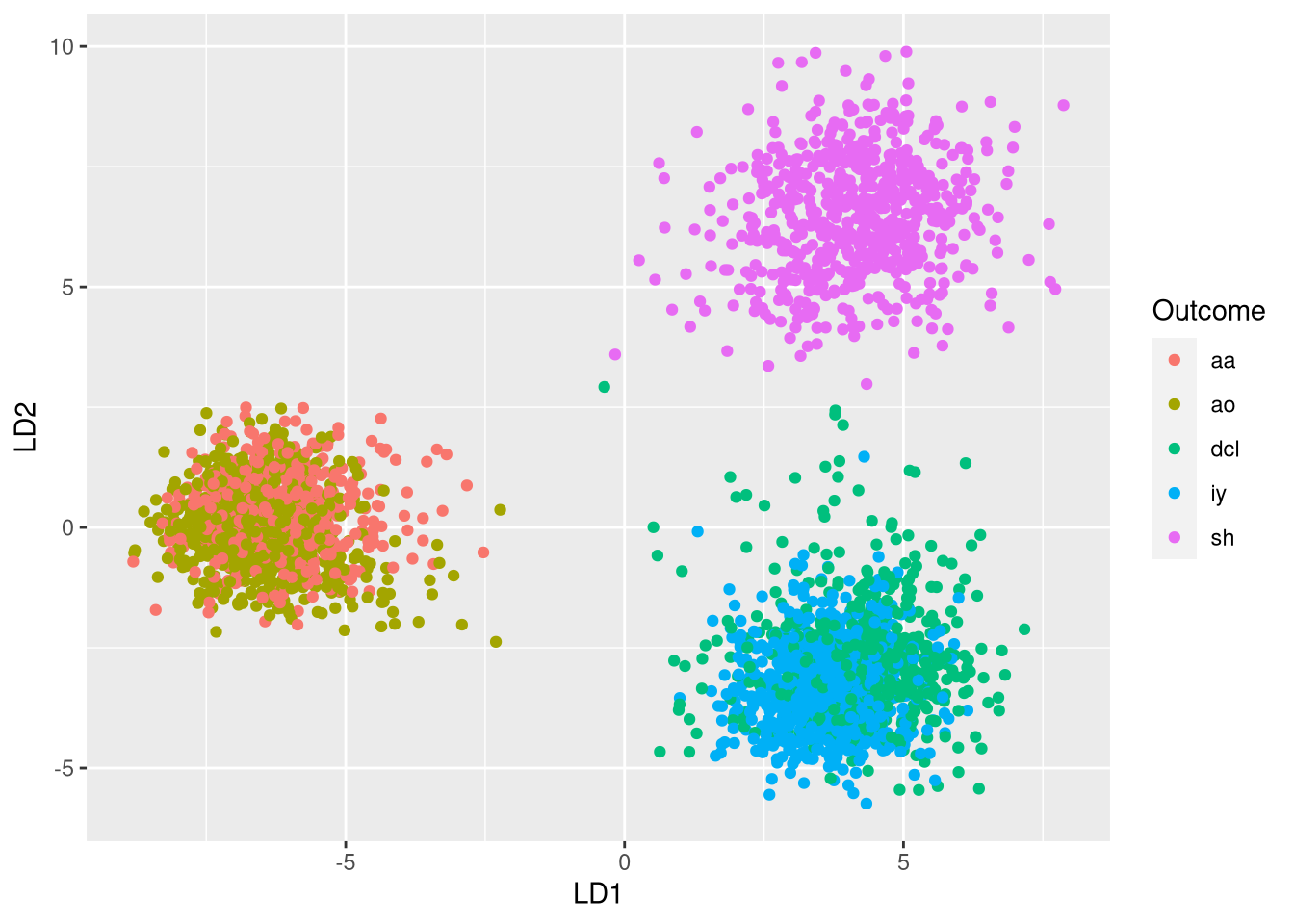
ggplot(plot.df, aes(x = LD1, y = LD2, color = Outcome)) + geom_point()
Plotting the data in the two LDA dimensions reveals three clusters:
- Cluster 1 (left) consists of aa and ao phonemes
- Cluster 2 (bottom right) consists of dcl and iy phonemes
- Cluster 3 (top right) consists of sh phonemes
This indicates that two dimensions are not sufficient for differentiating all 5 classes. However, the clustering indicates that phonemes that are sufficiently different from one another can be differentiated very well.
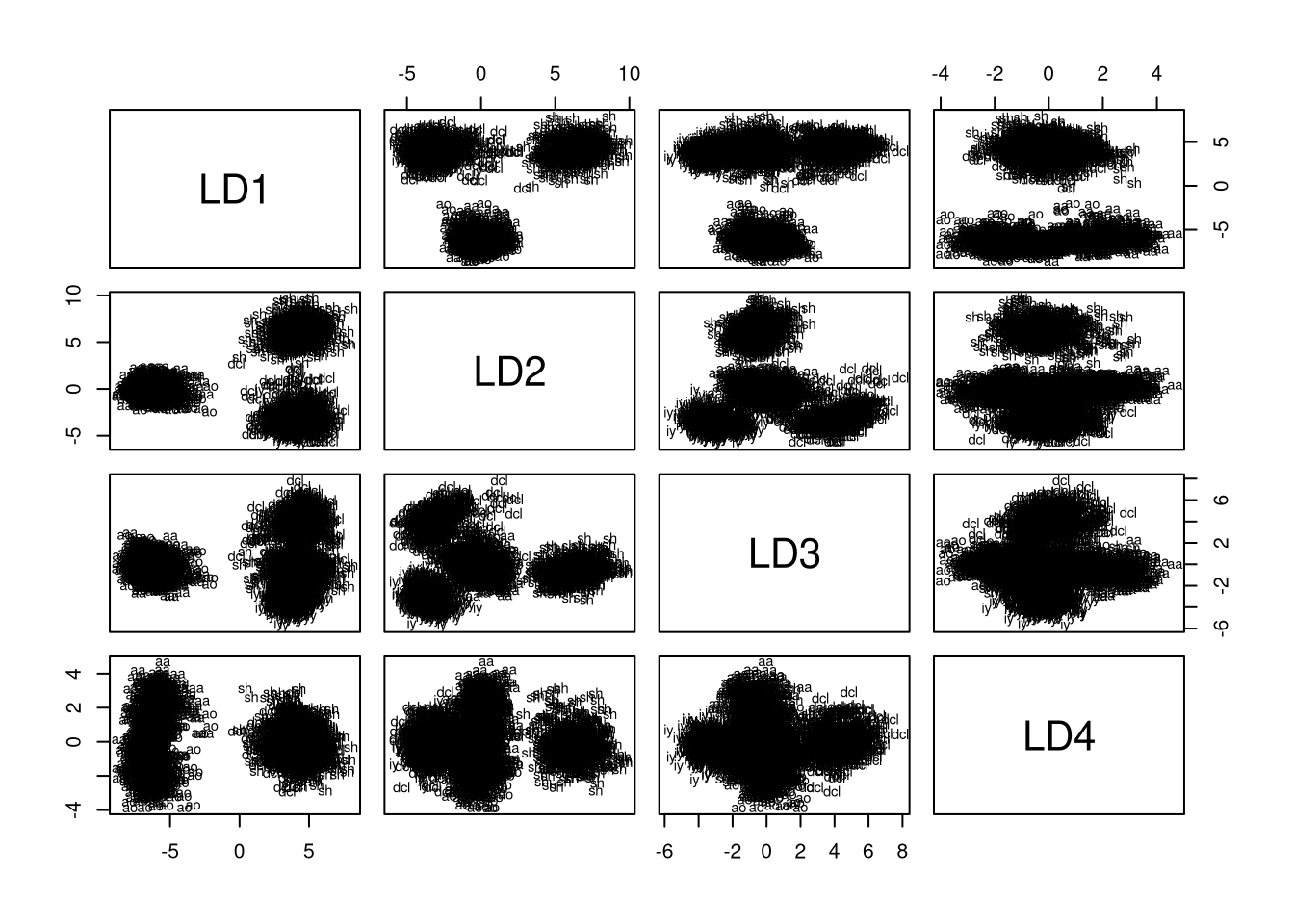
We can also plot the mapping of training data onto all pairs of discriminant variables using the plot.lda function where the dimen parameter can be used to specify the number of considered dimensions:
library(RColorBrewer)
colors <- brewer.pal(8, "Accent")
my.cols <- colors[match(lda.prediction.train$class, levels(df$g))]
plot(lda.model, dimen = 4, col = my.cols)
Plotting the training data for all dimension pairs demonstrates that, by construction, capture most of the variance. Using the plot, we can obtain an intuition about the number of dimensions we should select for reduced-rank LDA. Remember that LD1 and LD2 confused aa with ao and dcl with iy. Thus, we need additional dimensions for differentiating these groups. Looking at the plots, it seems that we indeed need all of the four dimensions because dcl and iy are only well-separated in LD1 vs LD3, while aa and ao are only well-separated when LD4 is combined with any of the other dimensions.
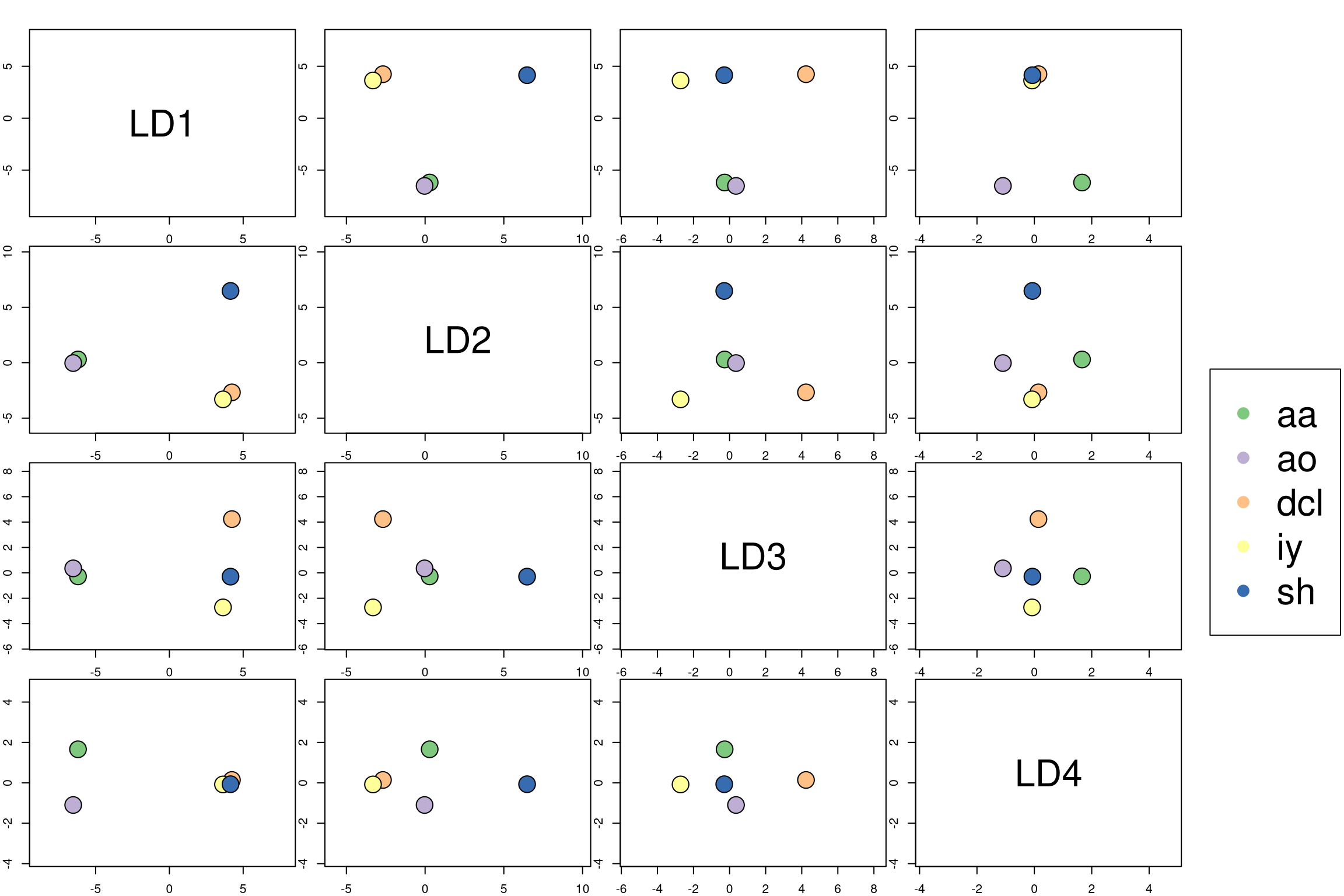
To visualize the centroids of the groups, we can create a custom plot:
plot_lda_centroids <- function(lda.model, train.set, response) {
    centroids <- predict(lda.model, lda.model$means)$x
    library(RColorBrewer)
    colors <- brewer.pal(8, "Accent")
    my.cols <- colors[match(lda.prediction.train$class, levels(df$g))]
    my.points <- predict(lda.model, train.set)$x
    no.classes <- length(unique(response))
    par(mfrow=c(no.classes -1, no.classes -1), mar=c(1,1,1,1), oma=c(1,1,1,10))
    for (i in 1:(no.classes - 1)) {
        for (j in 1:(no.classes - 1)) {
            y <- my.points[, i]
            x <- my.points[, j]
            cen <- cbind(centroids[, j], centroids[, i])
            if (i == j) {
                plot(x, y, type="n")
                max.y <- max(my.points[, i])
                max.x <- max(my.points[, j])
                min.y <- min(my.points[, i])
                min.x <- min(my.points[, j])
                max.both <- max(c(max.x, max.y))
                min.both <- max(c(min.x, min.y))
                center <- min.both + ((max.both - min.both) / 2)
                text(center, center, colnames(my.points)[i], cex = 3)}
            else {
                plot(x, y, col = my.cols, pch = as.character(response), xlab ="", ylab="")
                points(cen[,1], cen[,2], pch = 21, col = "black", bg = colors, cex = 3)
            }
        }
    }
    par(xpd = NA)
    legend(x=par("usr")[2] + 1, y = mean(par("usr")[3:4]) + 20,
            legend = rownames(centroids), col = colors, pch = rep(20, length(colors)), cex = 3)
}
plot_lda_centroids(lda.model, train.set, train.responses)
Interpreting the posterior probabilities
Besides the transformation of the data to the discriminant variables, which is provided by the component x, the predict function also gives the posterior probabilities, which can be used for further interpretation of the classifier. For example:
posteriors <- lda.prediction.train$posterior # N x K matrix
# MAP classification for sample 1:
pred.class <- names(which.max(posteriors[1,])) # <=> lda.prediction.train$class[1]
print(paste0("Posterior of predicted class '", pred.class,
"' is: ", round(posteriors[1,pred.class], 2)))## [1] "Posterior of predicted class 'sh' is: 1"# what are the mean posteriors for individual groups?
classes <- colnames(posteriors)
res <- do.call(rbind, (lapply(classes, function(x) apply(posteriors[train.responses == x, ], 2, mean))))
rownames(res) <- classes
print(round(res, 3)) ## aa ao dcl iy sh
## aa 0.797 0.203 0.000 0.000 0.000
## ao 0.123 0.877 0.000 0.000 0.000
## dcl 0.000 0.000 0.985 0.014 0.002
## iy 0.000 0.000 0.001 0.999 0.000
## sh 0.000 0.000 0.000 0.000 1.000The table of posteriors for individual classes demonstrates that the model is most uncertain about the phonemes aa and ao, which is in agreement with our expectations from the visualizations.
LDA as a classifier
As mentioned before, LDA has the benefit that we can select the number of canonical variables that are used for classification. Here, we will still showcase the use of reduced-rank LDA by performing classification with up to four canonical variables.
dims <- 1:4 # number of canonical variables to use
accuracies <- rep(NA, length(dims))
for (i in seq_along(dims)) {
    lda.pred <- predict(lda.model, test.set, dim = dims[i])
    acc <- length(which(lda.pred$class == test.responses))/length(test.responses)
    accuracies[i] <- acc
}
reduced.df <- data.frame("Rank" = dims, "Accuracy" = round(accuracies, 2))
print(reduced.df)## Rank Accuracy
## 1 1 0.51
## 2 2 0.71
## 3 3 0.86
## 4 4 0.92As expected from the visual exploration of the transformed space, the test accuracy increases with each additional dimension. Since LDA with four dimension obtains the maximal accuracy, we would decide to use all of the discriminant coordinates for classification.
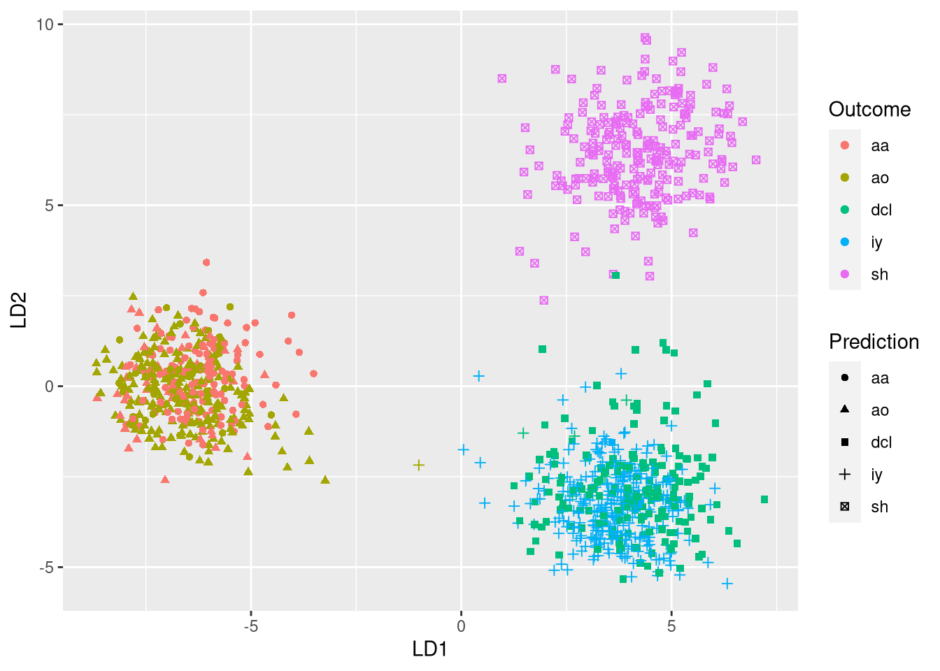
To interpret the model, we can visualize the performance of the full-rank classifier:
lda.pred <- predict(lda.model, test.set)
plot.df <- data.frame(lda.pred$x[,1:2], "Outcome" = test.responses,
                    "Prediction" = lda.pred$class)
ggplot(plot.df, aes(x = LD1, y = LD2, color = Outcome, shape = Prediction)) +
        geom_point()
In the plot, the expected phonemes are shown by different colors, while the model predictions are shown through different symbols. A model with 100% accuracy would assign a single symbol to each each color. Thus, incorrect predictions are revealed when a single color exhibits different symbols. Using the plot, we quickly see that most confusions occur when observations labeled as aa are incorrectly classified as ao and vice versa.
Quadratic discriminant analysis
QDA is a variant of LDA in which an individual covariance matrix is estimated for every class of observations. QDA is particularly useful if there is prior knowledge that individual classes exhibit distinct covariances. A disadvantage of QDA is that it cannot be used as a dimensionality reduction technique.
In QDA, we need to estimate Σk for each class k∈{1,…,K} rather than assuming Σk=Σ as in LDA. The discriminant function of LDA is quadratic in x:
δk(x)=−12log|Σk|−12(x−μk)TΣ−1k(x−μk)+logπk.
Since QDA estimates a covariance matrix for each class, it has a greater number of effective parameters than LDA. We can derive the number of parameters in the following way.
- We need K class priors πk. Since ∑Ki=1πk=1, we do not need a parameter for one of the priors. Thus, there are K−1 free parameters for the priors.
- Since there are K centroids, μk, with p entries each, there are Kp parameters relating to the means.
- From the covariance matrix, Σk, we only need to consider the diagonal and the upper right triangle. This region of the covariance matrix has p(p+1)2 elements. Since K such matrices need to be estimated, there are Kp(p+1)2 parameters relating to the covariance matrices.
Thus, the effective number of QDA parameters is K−1+Kp+Kp(p+1)2.
Since the number of QDA parameters is quadratic in p, QDA should be used with care when the feature space is large.
QDA in R
We can perform QDA in the following way:
qda.model <- qda(train.set, grouping = train.responses)The main difference between the QDA and the LDA object is that the QDA has a p×p transformation matrix for every class k∈{1,…,K}. These matrices ensure that the within-group covariance matrix is spherical but do not induce a reduced subspace. Thus, QDA cannot be used as a visualization technique.
Let us determine whether QDA outperforms LDA on the phoneme data set:
qda.preds <- predict(qda.model, test.set)
acc <- length(which(qda.preds$class == test.responses))/length(test.responses)
print(paste0("Accuracy of QDA is: " , round(acc, 2)))
## [1] "Accuracy of QDA is: 0.84"The accuracy of QDA is slightly below that of full-rank LDA. This could indicate that the assumption of common covariance is suitable for this data set.
Regularized discriminant analysis
RDA is a compromise between LDA and QDA as it shrinks Σk to a pooled variance Σ by defining
ˆΣk(α)=αˆΣk+(1−α)ˆΣ
and replacing ˆΣk with ˆΣk(α) in the discriminant functions. Here, α∈[0,1] is a tuning parameter determining whether the covariances should be estimated independently (α=1) or should be pooled (α=0).
Additionally, ˆΣ can also be shrunk toward the scalar covariance by requiring
ˆΣ(γ)=γˆΣ+(1−γ)ˆσ2I
where γ=1 leads to the pooled covariance and γ=0 leads to the scalar covariance. Replacing ˆΣk by ˆΣ(α,γ) leads to a more general notion of covariance.
Since RDA is a regularization technique, it is particularly useful when there are many features that are potentially correlated. Let us now evaluate RDA on the phoneme data set.
RDA in R
To perform RDA, we need to load the rda package. Note that rda was removed from CRAN, so you need to install it manually now (2020-07). A regularized discriminant analysis model can be fit using the rda function, which has two main parameters: α as introduced before and δ, which defines the threshold for values.
library(rda)
# note: optimization is time-intensive, especially if many alpha/gammas are used
alphas <- c(0.1, 0.25, 0.5, 0.75, 0.9)
rda.model <- rda(t(as.matrix(train.set)), y = train.responses,
                alpha = alphas)
Having obtained the fitted model, let us determine the performance of RDA on the test set. The following code is a bit more complicated than the code for LDA/QDA because we need to iterate over the results for both α and δ:
rda.preds <- predict(rda.model, t(train.set), train.responses, t(test.set))
# determine performance for each alpha:
rda.perf <- vector("list", dim(rda.preds)[1])
for (i in seq(dim(rda.preds)[1])) {
    # performance for each gamma
    res <- apply(rda.preds[i,,], 1, function(x) length(which(x == as.numeric(test.responses))) / length(test.responses))
    rda.perf[[i]] <- res
}
rda.perf <- do.call(rbind, rda.perf)
rownames(rda.perf) <- alphas
The calculated accuracies suggest that the RDA classifier with δ=0 and α=0.25 (92.2% accuracy) slightly outperforms full-rank LDA (91.9% accuracy).
Conclusions
Discriminant analysis is particularly useful for multi-class problems. LDA is very interpretable because it allows for dimensionality reduction. Using QDA, it is possible to model non-linear relationships. RDA is a regularized discriminant analysis technique that is particularly useful for large number of features. Besides these methods, there are also other techniques based on discriminants such as flexible discriminant analysis, penalized discriminant analysis, and mixture discriminant analysis.


Comments
Adamou Ibrahim M. Laouali
02 Dec 18 00:01 UTC
Matthias Döring
02 Dec 18 08:30 UTC
Renuka Vallabhanei
02 Dec 18 13:22 UTC