Interpreting Linear Prediction Models
Although linear models are one of the simplest machine learning techniques, they are still a powerful tool for predictions. This is particularly due to the fact that linear models are especially easy to interpret. Here, I discuss the most important aspects when interpreting linear models by example of ordinary least-squares regression using the airquality data set.
The airquality data set
The airquality data set contains 154 measurements of the following four air quality metrics as obtained in New York:
- Ozone: Mean ozone level in parts per billion
- Solar.R: Solar radiation in Langleys
- Wind: Average wind speed in miles per hour
- Temp: Maximum daily temperature in degrees Fahrenheit
We’ll clean up the data set by removing all NA entries and excluding the Month and Day columns, which should not play a role as predictors.
data(airquality)
ozone <- subset(na.omit(airquality),
        select = c("Ozone", "Solar.R", "Wind", "Temp"))
Data exploration and preparation
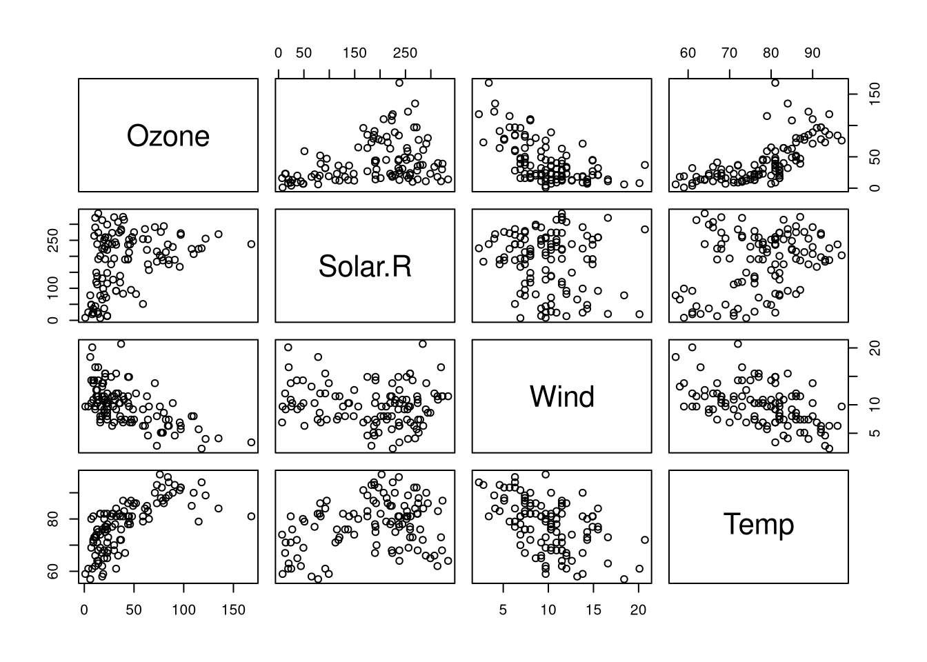
The prediction task is the following: Can we predict the ozone level given solar radiation, wind speed, and temperature? To see whether the assumptions of the linear model are appropriate for the data at hand, we will compute the correlation between the variables:
# scatterplot matrix
plot(ozone)
# pairwise variable correlations
cors <- cor(ozone)
print(cors)
## Ozone Solar.R Wind Temp
## Ozone 1.0000000 0.3483417 -0.6124966 0.6985414
## Solar.R 0.3483417 1.0000000 -0.1271835 0.2940876
## Wind -0.6124966 -0.1271835 1.0000000 -0.4971897
## Temp 0.6985414 0.2940876 -0.4971897 1.0000000# which variables are highly correlated, exclude self-correlation
cor.idx <- which(abs(cors) >= 0.5 & cors != 1, arr.ind = TRUE)
cor.names <- paste0(colnames(ozone)[cor.idx[,1]], "+",
colnames(ozone)[cor.idx[,2]], ": ", round(cors[cor.idx], 2))
print(cor.names)## [1] "Wind+Ozone: -0.61" "Temp+Ozone: 0.7" "Ozone+Wind: -0.61"
## [4] "Ozone+Temp: 0.7"Since ozone is involved in two linear interactions, namely:
- Ozone has a positive correlation with temperature
- Ozone has a negative correlation with wind
This suggests that it should be possible to form a linear model predicting the ozone level using the remaining features.
Splitting into training and test sets
We will take 70% of samples for training and 30% for testing:
set.seed(123)
N.train <- ceiling(0.7 * nrow(ozone))
N.test <- nrow(ozone) - N.train
trainset <- sample(seq_len(nrow(ozone)), N.train)
testset <- setdiff(seq_len(nrow(ozone)), trainset)
Investigating the linear model
To illustrate the most important aspects of interpreting linear models, we will train an ordinary least-squares model for the training data in the following way:
model <- lm(Ozone ~ Solar.R + Temp + Wind, ozone, trainset)To interpret the model, we use the summary function:
model.summary <- summary(model)
print(model.summary)##
## Call:
## lm(formula = Ozone ~ Solar.R + Temp + Wind, data = ozone, subset = trainset)
##
## Residuals:
## Min 1Q Median 3Q Max
## -29.913 -16.014 -3.949 7.818 92.987
##
## Coefficients:
## Estimate Std. Error t value Pr(>|t|)
## (Intercept) -74.18929 28.65268 -2.589 0.0116 *
## Solar.R 0.04507 0.02844 1.585 0.1173
## Temp 1.84999 0.31696 5.837 1.32e-07 ***
## Wind -3.34510 0.80164 -4.173 8.10e-05 ***
## ---
## Signif. codes: 0 '***' 0.001 '**' 0.01 '*' 0.05 '.' 0.1 ' ' 1
##
## Residual standard error: 22.25 on 74 degrees of freedom
## Multiple R-squared: 0.622, Adjusted R-squared: 0.6067
## F-statistic: 40.59 on 3 and 74 DF, p-value: 1.286e-15The residuals
The first piece of information we obtain is on the residuals. The term residual comes from the residual sum of squares (RSS), which is defined as
ri=yi−f(xi)RSS=n∑i=1r2i
where the residual ri is defined as the difference between observed and predicted values, f(xi), from the observed value, yi.
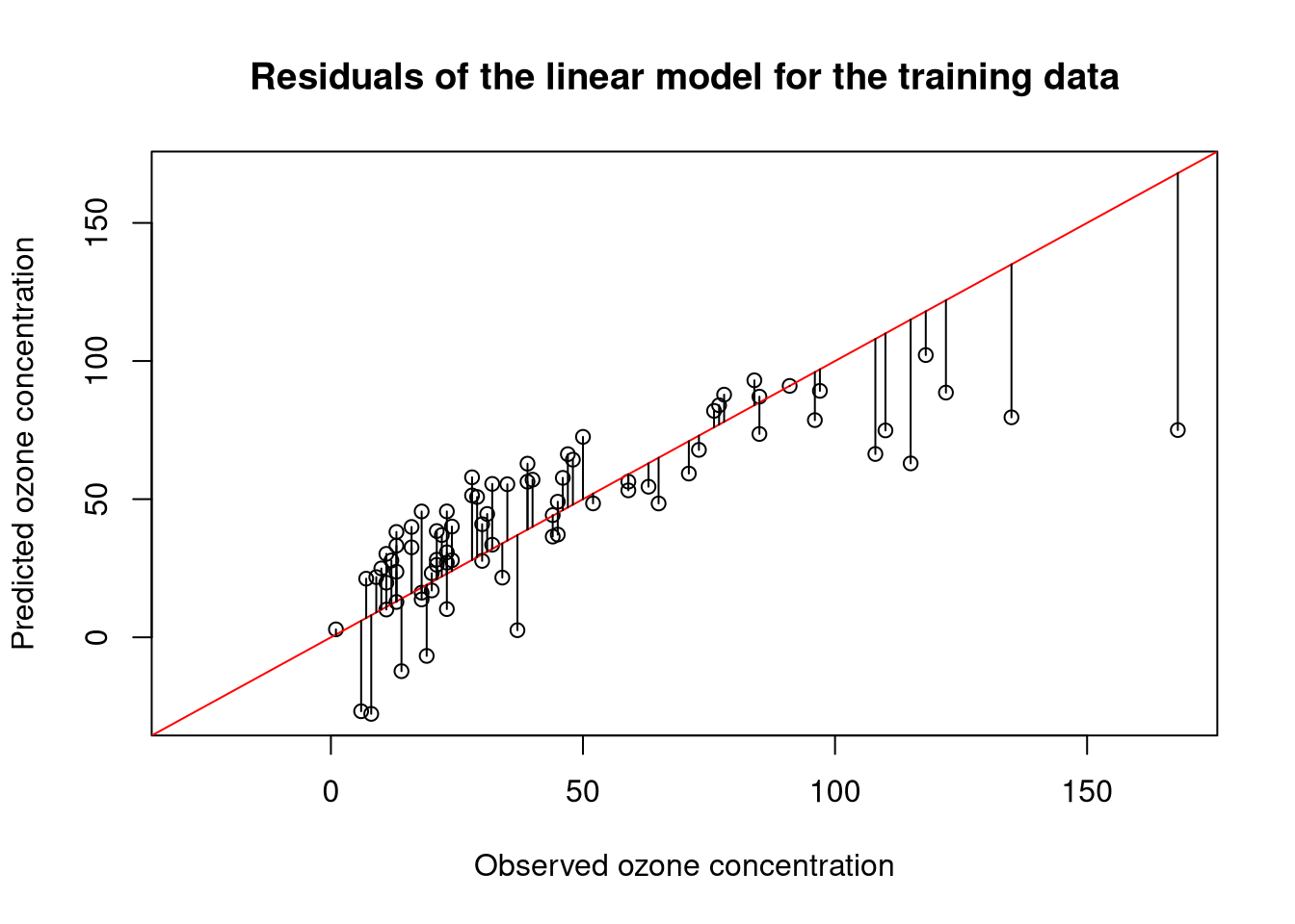
The residual median value suggest that the model generally predicts slightly higher values of ozone than observed. The large maximum value, however, indicates that some outlier predictions are also much too low. Looking at a numbers can be a bit abstract, so let us plot the predictions of the model against the observed values:
res <- residuals(model)
# ensure that x- and y-axis have the same range
pred <- model$fitted.values
obs <- ozone[trainset, "Ozone"]
# determine maximal range
val.range <- range(pred, obs)
plot(obs, pred,
    xlim = val.range, ylim = val.range,
    xlab = "Observed ozone concentration",
    ylab = "Predicted ozone concentration",
    main = "Residuals of the linear model for the training data")
# show ideal prediction as a diagonal
abline(0,1, col = "red")
# add residuals to the plot
segments(obs, pred, obs, pred + res)
The coefficients
Now that we understand the residuals, let’s take a look at the coefficients. We can use the coefficients function to obtain the fitted coefficients of the model:
coefficients(model)## (Intercept) Solar.R Temp Wind
## -74.18928801 0.04506998 1.84999289 -3.34510459Note that the intercept of the model has quite a low value. This is the value that the model will predict in the case that all independent values are zero. The low coefficient for Solar.R indicates that solar radiation does not play an important role for predicting ozone levels, which does not come as a surprise as it did not show a large correlation with the ozone level in our exploratory analysis. The coefficient for Temp indicates that ozone levels are high if the temperature is high (since ozone will form faster). The coefficient for Wind tells us that ozone levels will be low for fast winds (since ozone will be blown away).
The other values associated with the coefficients give information about the statistical certainty of the estimates.
model.summary$coefficients## Estimate Std. Error t value Pr(>|t|)
## (Intercept) -74.18928801 28.65267764 -2.589262 1.157483e-02
## Solar.R 0.04506998 0.02843762 1.584871 1.172601e-01
## Temp 1.84999289 0.31695917 5.836692 1.317712e-07
## Wind -3.34510459 0.80164181 -4.172817 8.103673e-05Std. Erroris the standard error of the coefficient estimatet valueindicates the value of the coefficient in terms of the standard errorPr(>|t|)is the p-value for the t-test, which indicates the significance of the test statistic
The standard error
The standard error of the coefficients is defined as the standard deviation of the feature variance:
ˆσ=√diag(σ2err(XTX)−1)
where XTX−1 is the inverse of the design matrix X, which includes the intercept, and where σ2err is the variance of the error.
In R, the standard errors of the model estimates can be computed via:
# compute variance-covariance matrix of model estimates
var.matrix <- vcov(model)
print(var.matrix)
## (Intercept) Solar.R Temp Wind
## (Intercept) 820.97593617 0.0787079320 -8.596270586 -16.239437823
## Solar.R 0.07870793 0.0008086984 -0.002707639 -0.002198751
## Temp -8.59627059 -0.0027076392 0.100463112 0.131551223
## Wind -16.23943782 -0.0021987513 0.131551223 0.642629584# use variances from variance-covariance matrix
std.err <- sqrt(diag(vcov(model)))
print(std.err)## (Intercept) Solar.R Temp Wind
## 28.65267764 0.02843762 0.31695917 0.80164181Now, you are probably wondering where the values from vcov are coming from. It is defined as the variance-covariance matrix of the design matrix scaled by the variance of the error:
scaled.var.matrix <- model.summary$cov.unscaled * model.summary$sigma^2
print(scaled.var.matrix)
## (Intercept) Solar.R Temp Wind
## (Intercept) 820.97593617 0.0787079320 -8.596270586 -16.239437823
## Solar.R 0.07870793 0.0008086984 -0.002707639 -0.002198751
## Temp -8.59627059 -0.0027076392 0.100463112 0.131551223
## Wind -16.23943782 -0.0021987513 0.131551223 0.642629584The variance that is used to scale to unscaled variance-covariance matrix is the estimated variance of the error, which is defined by
σ2err=1n−pRSS
The cov.unscaled parameter is simply the variance-covariance matrix of all features βi (including the intercept) of the design matrix:
# include intercept as a feature via 'model.matrix'
X <- model.matrix(model) # design matrix
# solve X^T %*% X = I to find the inverse of X^T * X
unscaled.var.matrix <- solve(crossprod(X), diag(4))
print(paste("Is this the same?", isTRUE(all.equal(unscaled.var.matrix, model.summary$cov.unscaled, check.attributes = FALSE))))## [1] "Is this the same? TRUE"The t-value
The t-value is defined as
ti=ˆβiˆσi
In R, they are computed via
# divide model coefficients by standard errors
t.vals <- coef(model) / std.err
print(t.vals)
## (Intercept) Solar.R Temp Wind
## -2.589262 1.584871 5.836692 -4.172817The p-value
The p-value is computed under the assumption that βi=0 for all coefficients. The t-values follow a t-distribution with
model.df <- df.residual(model)degrees of freedom. The degrees of freedom of a linear model is defined as
df=n−p
Further statistics
The following additional statistics are provided by the summary function: the multiple R-squared, the adjusted R-squared, and the F-statistic. A nice summary of these statistics is available at StackExchange.
Residual standard error
As the name suggests, the residual standard error is the square root of the mean RSS (MSE) of model:
rss <- sum(res^2)
mean.rss <- rss / model.df
res.std.error <- sqrt(mean.rss)
print(res.std.error)
## [1] 22.24615The residual standard error simply indicates the average accuracy of the model. In this case, the value is quite low, indicating that the model has a good fit.
The multiple R-squared
The multiple R-squared indicates the coefficient of determination. It is defined as the square of the correlation between estimates and observed outcomes:
r.squared <- cor(pred, obs)^2
print(r.squared)
## [1] 0.6219815In contrast to the correlation, which is in [−1,1], R-squared is in [0,1].
The adjusted R-squared
The adjusted R-squared value adjusts the R-squared according to the complexity of the model:
R2a=1−(1−R2)n−1n−p−1
where n is the number of observations and p the number of features. Thus, the adjusted R-squared can be computed like this:
n <- length(trainset) # number of samples
p <- length(coefficients(model)) - 1 # number of features w/o intercept
r.squared.adj <- 1 - (1 - r.squared) * ((n - 1) / (n - p - 1))
print(r.squared.adj)
## [1] 0.6066564If there is a considerable difference between R-squared and the adjusted R-squared, this indicates that one may consider reducing the feature space.
The F-statistic
The F-statistic is defined as the ratio of explained vs unexplained variance. For regression, the F-statistic always indicates the difference between two models where model 1 (p1) is defined by a subset of features from model 2 (p2):
F=(RSS1−RSS2p2−p1)(RSS2n−p2)
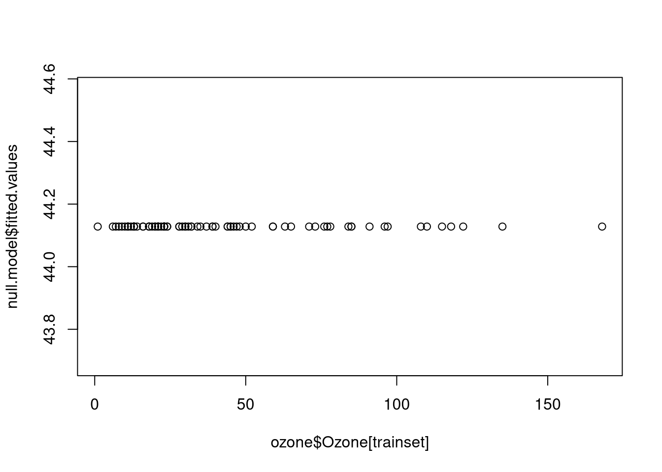
The F-statistic describes the extent to which the predictive performance (in terms of the RSS) of model 2 is superior over model 1. The default F-statistic that is reported refers to the difference between the trained model and the intercept-only model:
# create intercept-only model
null.model <- lm(formula = Ozone ~ 1, ozone, trainset)
print(null.model)##
## Call:
## lm(formula = Ozone ~ 1, data = ozone, subset = trainset)
##
## Coefficients:
## (Intercept)
## 44.13# plot the incercept-only prediction function
plot(ozone$Ozone[trainset], null.model$fitted.values) Hence, the null hypothesis of the test is that the fit of the intercept-only model and the specified model is equal. If the null hypothesis can be rejected, this implies that the specified model has a better fit than the null model.
Let’s calculate this by hand to show the idea:
rss <- function(model) {
    return(sum(model$residuals^2))
}
f.statistic <- function(model1, model2) {
    n <- length(model1$fitted.values)
    n2 <- length(model2$fitted.values)
    if (n != n2) {
        stop("Both models should have the same number of training samples!")
    }
    p1 <- length(coefficients(model1))
    p2 <- length(coefficients(model2))
    enum <- (rss(model1) - rss(model2)) / (p2 - p1)
    denom <- rss(model2) / (n - p2)
    out <- enum/denom
    return(out)
}
# compare the intercept-only model and the model with 3 features
f.statistic(null.model, model)
## [1] 40.58587In this case, the F-statistic has a large value, which indicates that we the trained model is significantly better than an intercept-only model.
Confidence intervals
Confidence intervals are a useful tool for interpreting linear models. By default, confint computes the 95% confidence interval (±1.96ˆσ):
ci <- confint(model)
apply(ci, 1, function(x) paste0("95% CI: [",
round(x[1], 2), ",", round(x[2], 2), "]"))## (Intercept) Solar.R Temp
## "95% CI: [-131.28,-17.1]" "95% CI: [-0.01,0.1]" "95% CI: [1.22,2.48]"
## Wind
## "95% CI: [-4.94,-1.75]"These values indicate that the model is quite unsure about the estimate of the intercept. This could suggest that more data is necessary to obtain a better fit.
Retrieving confidence and prediction intervals for estimated values
The predictions from a linear model can be turned into intervals by providing the interval argument. These intervals give a measure of confidence for the predicted values. There are two types of intervals: confidence and prediction intervals. Let’s apply our model on the test set using different arguments for the interval parameter to see the difference between the two types of intervals:
# compute confidence intervals (CI) for predictions:
preds.ci <- predict(model, newdata = ozone[testset,], interval = "confidence")
# compute prediction intervals (PI) for predictions:
preds.pred <- predict(model, newdata = ozone[testset,], interval = "prediction")
# note that the values differ:
cbind(rbind(preds.ci[1,], preds.pred[2,]), "Method" = c("CI", "PI"))## fit lwr upr Method
## [1,] "33.569757038475" "22.77849338542" "44.36102069153" "CI"
## [2,] "37.5676204778478" "-7.48876887421986" "82.6240098299155" "PI"The confidence intervals are narrow intervals, while the prediction (tolerance) intervals are wide intervals. Their values are based on the provided tolerance/significance level, as specified by the level parameter (default: 0.95).
Their definitions are slightly different. Given a new observation x, CIs and PIs are defined as follows
ˆyCI±tα/2,df√MSE⋅(1n(x−¯x)2∑i(xi−¯x)2)
where tα/2,df is the t-value with df=2 degrees of freedom and a significance level of α, σerr is the standard error of the residual, σ2x is the variance of the independent features, and ¯x indicates the mean value of the features. More detailed explanations for calculating CIs and PIs are available at RPubs and through this video.
With regard to their interpretation, the difference between the two intervals is further discussed at GraphPad.


Comments
There aren't any comments yet. Be the first to comment!