An Introduction to Probabilistic Programming with Stan in R
Probabilistic programming enables us to implement statistical models without having to worry about the technical details. It is particularly useful for Bayesian models that are based on MCMC sampling. In this article, I investigate how Stan can be used through its implementation in R, RStan. This post is largely based on the GitHub documentation of Rstan and its vignette.
Introduction to Stan
Stan is a C++ library for Bayesian inference. It is based on the No-U-Turn sampler (NUTS), which is used for estimating the posterior distribution according to a user-specified model and data. Performing an analysis using Stan involves the following steps:
- Specify the statistical model using the the Stan modeling language. This is typically done through a dedicated .stan file.
- Prepare the data that is to be fed to the model.
- Sample from the posterior distribution using the
stanfunction. - Analyze the results.
In this article, I will showcase the use of Stan using two hierarchical models. I will use the first model to talk about the basic features of Stan and the second example to demonstrate a more advanced application.
The eight schools data set
The first data set we are going to use is the eight schools data set (Rubin, 1981 and Gelman, 2003). This data set measures the effect of coaching programs on college admission tests, the scholastic aptitude test (SAT), which is used in the US. The SAT was designed in such a way that it should be resistant to short-term efforts directly targeted at improving the score in the test. Rather, the test should reflect the knowledge that was acquired over a longer period of time. The data set looks as follows:
| School | Estimated effect of coaching (yj) | Standard error of effect (σj) |
|---|---|---|
| A | 28 | 15 |
| B | 8 | 10 |
| C | -3 | 16 |
| D | 7 | 11 |
| E | -1 | 9 |
| F | 1 | 11 |
| G | 18 | 10 |
| H | 12 | 18 |
As we can see, the SAT did not fulfill its promise: for most of the eight schools, the short-term coaching indeed increased the SAT scores as evidenced by positive values of yj, where yj indicates the change in SAT scores. For this data set, we are interested in estimating the true effect size associated with each school. There are two alternative approaches that could be used. First, we could assume that all schools are independent of each other. However, this would lead to estimates that are hard to interpret because the 95% posterior intervals for the schools would largely overlap due to the high standard error. Second, one could pool the data from all schools, assuming that the true effect is the same in all schools. This, however, is also not reasonable because there should be school-specific effects (e.g. different teachers and students).
Thus, another model is required. The hierarchical model has the advantage of combining information from all eight schools (experiments) without assuming that they have common true effects. We can specify a hierarchial Bayesian model in the following way:
yi∼Normal(θj,σj),j=1,…,8Prior distributionθj∼Normal(μ,τ),j=1,…,8Posterior distributionp(μ,τ)∝1Parameter distribution is uniform
According to the model, the effects of coaching follow a normal distribution whose mean is the true effect, θj, and whose standard deviation is σj, which is known from the data. The true effect, θj, follows a normal distribution with parameters μ and τ.
Defining the Stan model file
Having specified the model we are going to use, we can now deliberate about how to specify this model in Stan. Before defining the Stan program for the model specified above, let us take a look at the structure of the Stan modeling language.
Variables
In Stan, variables can be defined in the following way:
int<lower=0> n; # lower bound is 0
int<upper=5> n; # upper bound is 5
int<lower=0,upper=5> n; # n is in [0,5]
Note that the upper and lower boundaries of the variables should be specified, if they are known a priori.
Multi-dimensional data can be specified via square brackets:
vector[n] numbers; // a vector of length n
real[n] numbers;  // an array of floats with length n
matrix[n,n] matrix; // an n times n matrix
Program blocks
The following program blocks are used in Stan:
- data: for specifying the data that is conditioned upon using Bayes rule
- transformed data: for preprocessing the data
- parameters (required): for specifying the parameters of the model
- transformed parameters: for parameter processing before computing the posterior
- model (required): for specifying the model itself
- generated quantities: for postprocessing the results
For the model program block, distributions can be specified in two equivalent ways. The first one, uses the following statistical notation:
y ~ normal(mu, sigma); # y follows a normal distributionThe second way uses a programmatic notation based on the log probability density function (lpdf):
target += normal_lpdf(y | mu, sigma); # increment the normal log densityStan supports a large number of probability distributions. When specifying models via Stan, the lookup function comes in handy: It provides a mapping from R functions to Stan functions. Consider the following example:
library(rstan) # load stan package
lookup(rnorm)## StanFunction Arguments ReturnType Page
## 355 normal_rng (real mu, real sigma) real 494Here, we see that the equivalent of rnorm in R is normal_rng in Stan.
The eight schools model
Now that we know the basics of the Stan modeling langeu, we can define our model, which we will store in a file called schools.stan:
data {
  int<lower=0> n; //number of schools
  real y[n]; // effect of coaching
  real<lower=0> sigma[n]; // standard errors of effects
}
parameters {
  real mu;  // the overall mean effect
  real<lower=0> tau; // the inverse variance of the effect
  vector[n] eta; // standardized school-level effects (see below)
}
transformed parameters {
  vector[n] theta;
  theta = mu + tau * eta; // find theta from mu, tau, and eta
}
model {
  target += normal_lpdf(eta | 0, 1); // eta follows standard normal
  target += normal_lpdf(y | theta, sigma);  // y follows normal with mean theta and sd sigma
}
Note that θ never appears in the parameters. This is because we do not explicitly model θ but instead model η, the standardized effect for individual schools. We then construct θ in the transformed parameters section according to μ, τ, and η. This parameterization makes the sampler more efficient.
Note that the model is specified using vector notation since both θ and σ indicate vectors. This allows for improved runtimes because it is not necessary to loop over every individual element.
Preparing the data for modeling
Before we can fit the model, we need to encode the input data as a list whose parameters should correspond to the entries in the data section of the Stan model. For the schools data, the data are the following:
schools.data <- list(
  n = 8,
  y = c(28,  8, -3,  7, -1,  1, 18, 12),
  sigma = c(15, 10, 16, 11,  9, 11, 10, 18)
)
Sampling from the posterior distribution
We can sample from the posterior distribution using the stan function, which performs the following three steps:
- It translate the model specification to C++ code.
- It compiles the C++ code to a shared object.
- It samples from the posterior distribution according to the specified model, data, and settings.
If rstan_options(auto_write = TRUE) has been executed in the active R session, subsequent calls of the same model will be much faster than the first call because the stan function then skips the first two steps (translating and compiling the model). Additionally, we will set the number of cores to be used:
options(mc.cores = parallel::detectCores()) # parallelize
rstan_options(auto_write = TRUE)  # store compiled stan model
Now, we can compile the model and sample from the posterior. The only two required parameters of stan are the location of the model file and the data to be fed to the model. The other parameters indicated here are just shown to provide an overview of the possible options:
fit1 <- stan(
  file = "schools.stan",  # Stan program
  data = schools.data,    # named list of data
  chains = 4,             # number of Markov chains
  warmup = 1000,          # number of warmup iterations per chain
  iter = 2000,            # total number of iterations per chain
  refresh = 1000          # show progress every 'refresh' iterations
  )
Model interpretation
We will first do a basic interpretation of the model and then investigate the MCMC procedure.
Basic model interpretation
To perform inference using the fitted model, we can use the print function.
print(fit1) # optional parameters: pars, probs## Inference for Stan model: schools.
## 4 chains, each with iter=2000; warmup=1000; thin=1;
## post-warmup draws per chain=1000, total post-warmup draws=4000.
##
## mean se_mean sd 2.5% 25% 50% 75% 97.5% n_eff Rhat
## mu 7.67 0.15 5.14 -2.69 4.42 7.83 10.93 17.87 1185 1
## tau 6.54 0.16 5.40 0.31 2.52 5.28 9.05 20.30 1157 1
## eta[1] 0.42 0.01 0.92 -1.47 -0.18 0.44 1.03 2.18 4000 1
## eta[2] 0.03 0.01 0.87 -1.74 -0.54 0.03 0.58 1.72 4000 1
## eta[3] -0.18 0.02 0.92 -1.95 -0.81 -0.20 0.45 1.65 3690 1
## eta[4] -0.03 0.01 0.92 -1.85 -0.64 -0.02 0.57 1.81 4000 1
## eta[5] -0.33 0.01 0.86 -2.05 -0.89 -0.34 0.22 1.43 3318 1
## eta[6] -0.20 0.01 0.87 -1.91 -0.80 -0.21 0.36 1.51 4000 1
## eta[7] 0.37 0.02 0.87 -1.37 -0.23 0.37 0.96 2.02 3017 1
## eta[8] 0.05 0.01 0.92 -1.77 -0.55 0.05 0.69 1.88 4000 1
## theta[1] 11.39 0.15 8.09 -2.21 6.14 10.30 15.56 30.22 2759 1
## theta[2] 7.92 0.10 6.25 -4.75 4.04 8.03 11.83 20.05 4000 1
## theta[3] 6.22 0.14 7.83 -11.41 2.03 6.64 10.80 20.97 3043 1
## theta[4] 7.58 0.10 6.54 -5.93 3.54 7.60 11.66 20.90 4000 1
## theta[5] 5.14 0.10 6.30 -8.68 1.40 5.63 9.50 16.12 4000 1
## theta[6] 6.08 0.10 6.62 -8.06 2.21 6.45 10.35 18.53 4000 1
## theta[7] 10.60 0.11 6.70 -0.94 6.15 10.01 14.48 25.75 4000 1
## theta[8] 8.19 0.14 8.18 -8.13 3.59 8.01 12.48 25.84 3361 1
## lp__ -39.47 0.07 2.58 -45.21 -41.01 -39.28 -37.70 -34.99 1251 1
##
## Samples were drawn using NUTS(diag_e) at Thu Nov 29 11:17:50 2018.
## For each parameter, n_eff is a crude measure of effective sample size,
## and Rhat is the potential scale reduction factor on split chains (at
## convergence, Rhat=1).Here, the row names indicate the estimated parameters: mu is the mean of the posterior distribution and tau is its standard deviation. The entries for eta and theta indicate the estimates for the vectors η and θ, respectively. The lp entry shows the log density, which is typically not relevant. The columns indicate the computed values. The percentages indicate the credible intervals. For example, the 95% credible interval for the overall effect of coaching, μ, is [−1.27,18.26]. Since we are not very certain of the mean, the 95% credible intervals for θj are also quite wide. For example, for the first school, the 95% credible interval is [−2.19,32.33].
We can visualize the uncertainty in the estimates using the plot function:
# specify the params to plot via pars
plot(fit1, pars = "theta")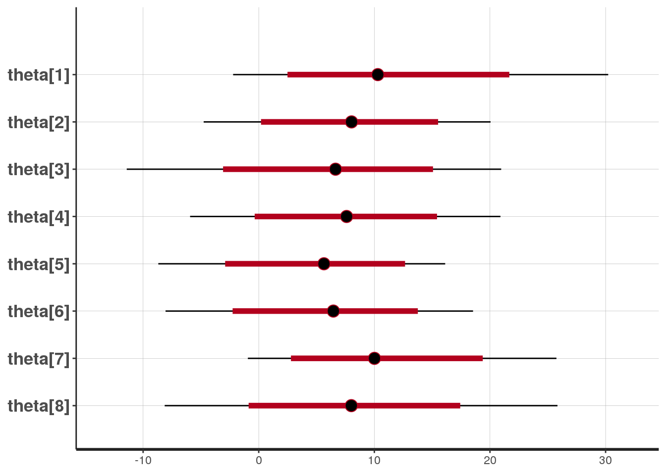
The black lines indicate the 95% intervals, while the red lines indicate the 80% intervals. The circles indicate the estimate of the mean.
We can obtain the generated samples using the extract function:
# retrieve the samples
samples <- extract(fit1, permuted = TRUE) # 1000 samples per parameter
mu <- samples$mu  # samples of mu only
MCMC diagnostics
There are also functions for diagnosing the MCMC procedure. By plotting the trace of the sampling procedure, we can identify whether anything has gone wrong during sampling. This could for example be the case if the chain stays in one place for too long or makes too many steps in one direction. We can plot the traces of the four chains used in our model with the traceplot function:
# diagnostics:
traceplot(fit1, pars = c("mu", "tau"), inc_warmup = TRUE, nrow = 2)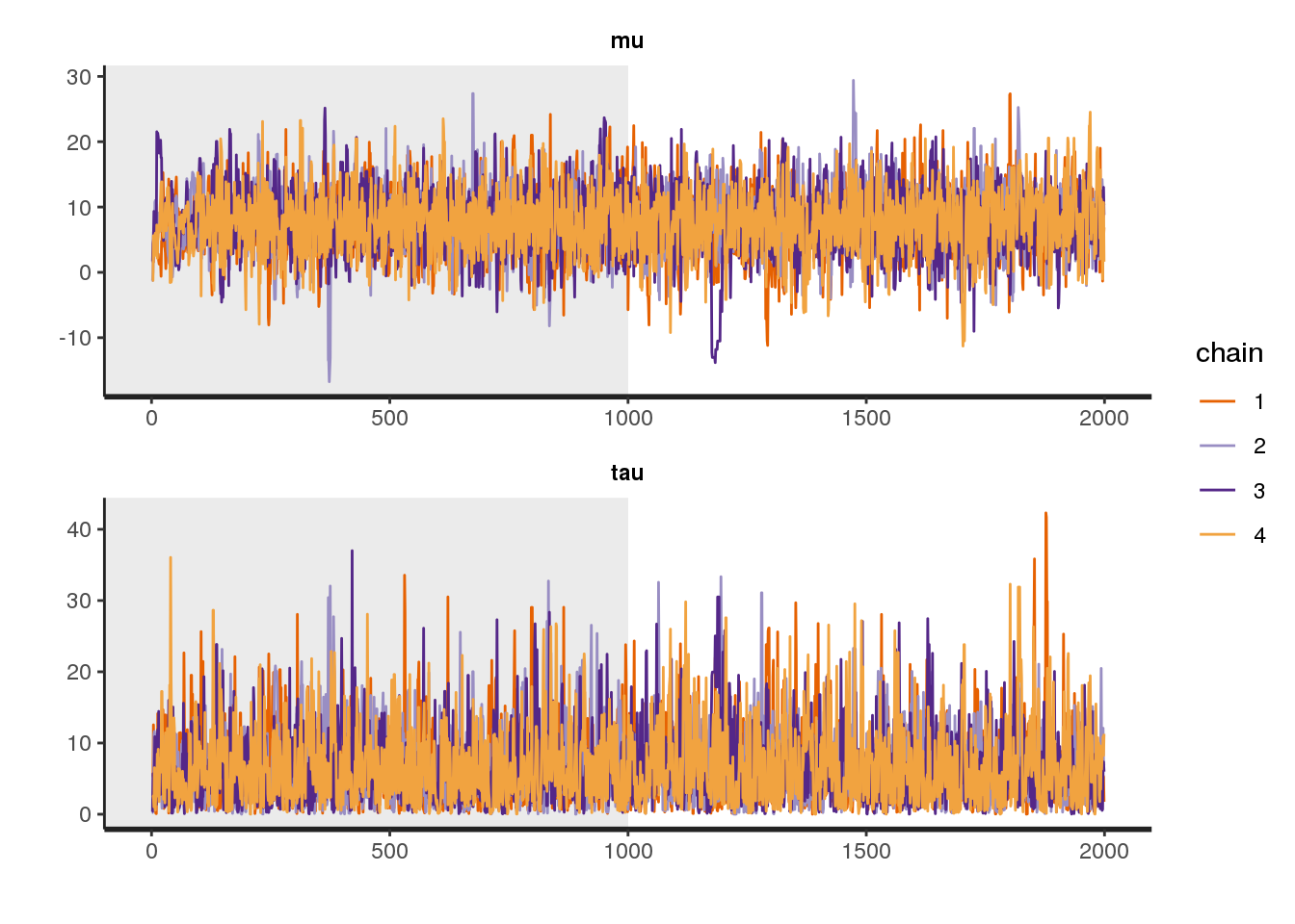
Both traces look fine to me.
To obtain the samples from individual Markov chains, we can use the extract function once again:
# retrieve matrix of iterations, chains, and parameters
chain.data <- extract(fit1, permuted = FALSE)
print(chain.data[1,,]) # parameters of all chains for the 1st of 1000 iterations
## parameters
## chains mu tau eta[1] eta[2] eta[3] eta[4]
## chain:1 1.111120 2.729124 -0.1581242 -0.8498898 0.5025965 -1.9874554
## chain:2 3.633421 2.588945 1.2058772 -1.1173221 1.4830778 0.4838649
## chain:3 13.793056 3.144159 0.6023924 -1.1188243 -1.2393491 -0.6118482
## chain:4 3.673380 13.889267 -0.0869434 1.1900236 -0.0378830 -0.2687284
## parameters
## chains eta[5] eta[6] eta[7] eta[8] theta[1]
## chain:1 0.3367602 -1.1940843 0.5834020 -0.08371249 0.6795797
## chain:2 -1.8057252 0.7429594 0.9517675 0.55907356 6.7553706
## chain:3 -1.5867789 0.6334288 -0.4613463 -1.44533007 15.6870727
## chain:4 0.1028605 0.3481214 0.9264762 0.45331024 2.4657999
## parameters
## chains theta[2] theta[3] theta[4] theta[5] theta[6] theta[7]
## chain:1 -1.208335 2.482769 -4.31289292 2.030181 -2.147684 2.703297
## chain:2 0.740736 7.473028 4.88612054 -1.041502 5.556902 6.097494
## chain:3 10.275294 9.896345 11.86930758 8.803971 15.784656 12.342510
## chain:4 20.201935 3.147213 -0.05906019 5.102037 8.508530 16.541455
## parameters
## chains theta[8] lp__
## chain:1 0.8826584 -41.21499
## chain:2 5.0808317 -41.17178
## chain:3 9.2487083 -40.35351
## chain:4 9.9695268 -36.34043To perform more advanced analytics of the sampling process, we can use the shinystan package, which provides a Shiny frontend. Using the package, a fitted model can be analyzed by starting the Shiny application in the following way:
library(shinystan)
launch_shinystan(fit1)
Hierarchical regression
Now that we have a basic understanding of Stan, we can dive into a more advanced application: Let’s try our hands at hierarchical regression. In conventional regression, we model a relationship of the form
Y=β0+Xβ.
This representation assumes that all samples have the same distribution. If there is a grouping of samples, then we have a problem because latent differences within and between groups will be ignored.
An alternative would be to have one regression model for each group. In this case, however, the small sample size would be problematic when estimating the individual models.
Hierarchical regression is a compromise between both extremes. This model assumes that the groups are similar but yet exhibit differences.
Assume that each sample belongs to one of K groups. Then, hierarchical regression is specified as follows:
Yk=αk+Xkβ(k),∀k∈{1,…,K}
where Yk is the outcome for the k-th group, αk is the intercept, Xk are the features, and β(k) indicates the weights. The hierarchical model is different from a model where Yk is fit for each group individually because the parameters, αk and β(k) are assumed to originate from a common distribution.
The rats data set
A classic example for hierarchical regression is the rats data set. This longitudinal data set contains the weights of rats as measured for 5 weeks. Let us load the data:
library(RCurl)
# load data as character
f <- getURL('https://www.datascienceblog.net/data-sets/rats.txt')
# read table from text connection
df <- read.delim(textConnection(f), header=T, sep = " ")
print(head(df)) # each row corresponds to an individual rat## day8 day15 day22 day29 day36
## 1 151 199 246 283 320
## 2 145 199 249 293 354
## 3 147 214 263 312 328
## 4 155 200 237 272 297
## 5 135 188 230 280 323
## 6 159 210 252 298 331Let us investigate the data:
library(reshape2)
ddf <- cbind(melt(df), Group = rep(paste0("Rat", seq(1, nrow(df))), 5))
library(ggplot2)
ggplot(ddf, aes(x = variable, y = value, group = Group)) + geom_line() + geom_point()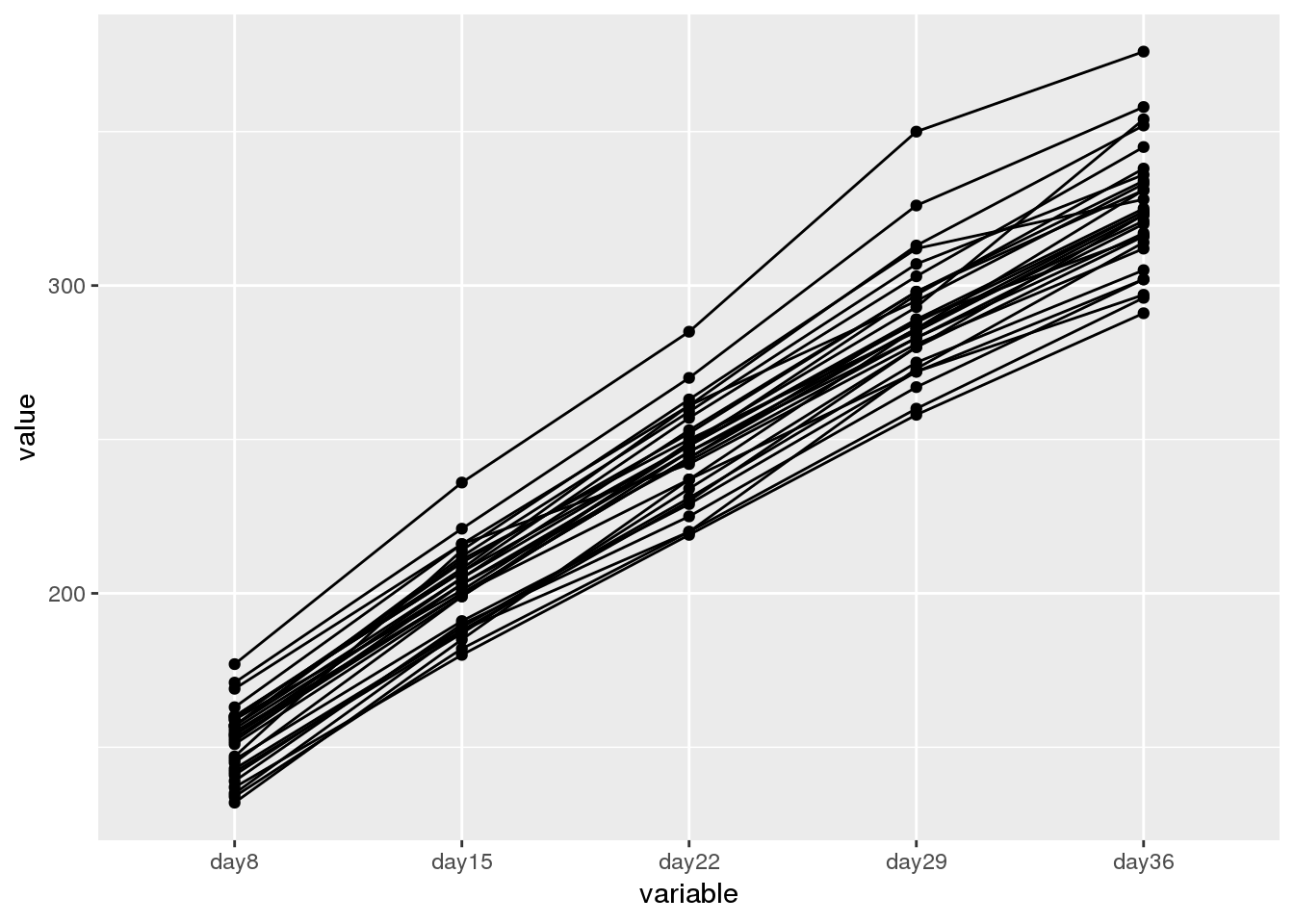
The data show a linear growth trend that is quite similar for different rats. However, we also see that the rats have different initial weights, which require different intercepts, as well as different growth rates, which require different slopes. Thus, a hierarchical model seems appropriate.
Specification of the hierarchical regression model
The model can be specified as follows:
Yij∼Normal(αi+βi(xj−ˉx),σY)αi∼Normal(μα,σα)βi∼Normal(μβ,σβ)
where the intercept for the i-th rat is indicated by αi and the slope by βi. Note that the measurement times are centered around ˉx=22 is the median measurement (day 22) of the time-series data.
We can now specify the model and store it in a file called rats.stan:
data {
    int<lower=0> N; // the number of rats
    int<lower=0> T; // the number of time points
    real x[T]; // day at which measurement was taken
    real y[N,T]; // matrix of weight times time
    real xbar; // the median number of days in the time series
}
parameters {
  real alpha[N]; // the intercepts of rat weights
  real beta[N]; // the slopes of rat weights

  real mu_alpha; // the mean intercept
  real mu_beta; // the mean slope

  real<lower=0> sigmasq_y;
  real<lower=0> sigmasq_alpha;
  real<lower=0> sigmasq_beta;
}
transformed parameters {
  real<lower=0> sigma_y; // sd of rat weight
  real<lower=0> sigma_alpha; // sd of intercept distribution
  real<lower=0> sigma_beta; // sd of slope distribution

  sigma_y <- sqrt(sigmasq_y);
  sigma_alpha <- sqrt(sigmasq_alpha);
  sigma_beta <- sqrt(sigmasq_beta);
}
model {
  mu_alpha ~ normal(0, 100); // non-informative prior
  mu_beta ~ normal(0, 100); // non-informative prior
  sigmasq_y ~ inv_gamma(0.001, 0.001); // conjugate prior of normal
  sigmasq_alpha ~ inv_gamma(0.001, 0.001); // conjugate prior of normal
  sigmasq_beta ~ inv_gamma(0.001, 0.001); // conjugate prior of normal
  alpha ~ normal(mu_alpha, sigma_alpha); // all intercepts are normal
  beta ~ normal(mu_beta, sigma_beta);  // all slopes are normal
  for (n in 1:N) // for each sample
    for (t in 1:T)  // for each time point
      y[n,t] ~ normal(alpha[n] + beta[n] * (x[t] - xbar), sigma_y);

}
generated quantities {
  // determine the intercept at time 0 (birth weight)
  real alpha0;
  alpha0 <- mu_alpha - xbar * mu_beta;
}
Note that the model code estimates the variance (the sigmasq variables) rather than the standard deviations. Additionally, the generated quantities block explicitly calculates α0, the intercept at time 0, that is, the weight of the rats at birth. We could have also calculated any other quantity in the generated quantities block, for example, the estimated weight of the rats at different points in time. We will do this in R later.
Data preparation
To prepare the data for the model, we first extract the measurement points as numeric values and then encode everything in a list structure:
days <- as.numeric(regmatches(colnames(df), regexpr("[0-9]*$", colnames(df))))
rat.data <- list(N = nrow(df), T = ncol(df), x = days,
                 y = df, xbar = median(days))
Fitting the regression model
We can now fit the Bayesian hierarchical regression model for the rat weight data set:
rat.model <- stan(
  file = "rats.stan",
  data = rat.data)
# model contains estimates for intercepts (alpha) and slopes (beta)
Prediction with the hiearchical regression model
Having determined α and β for each rat, we can now estimate the weight of individual rats at arbitrary points in time. Here, we are interested in finding the weight of the rats from day 0 to day 100.
predict.rat.weight <- function(rat.model, newdays) {
    # newdays: vector of time points to consider
    rat.fit <- extract(rat.model)
    alpha <- rat.fit$alpha
    beta <- rat.fit$beta
    xbar <- 22 # hardcoded since not stored in rat.model
    y <- lapply(newdays, function(t) alpha + beta * (t - 22))
    return(y)
}
newdays <- seq(0, 100)
pred.weights <- predict.rat.weight(rat.model, newdays)
# extract means and standard deviations from posterior samples
pred.means <- lapply(pred.weights, function(x) apply(x, 2, mean))
pred.sd <- lapply(pred.weights, function(x) apply(x, 2, sd))
# create plotting data frame with 95% CI interval from sd
pred.df <- data.frame(Weight = unlist(pred.means),
              Upr_Weight = unlist(pred.means) + 1.96 * unlist(pred.sd),
              Lwr_Weight = unlist(pred.means) - 1.96 * unlist(pred.sd),
              Day = unlist(lapply(newdays, function(x) rep(x, 30))),
              Rat = rep(seq(1,30), length(newdays)))
# predicted mean weight of all rats
ggplot(pred.df, aes(x = Day, y = Weight, group = Rat)) +
    geom_line()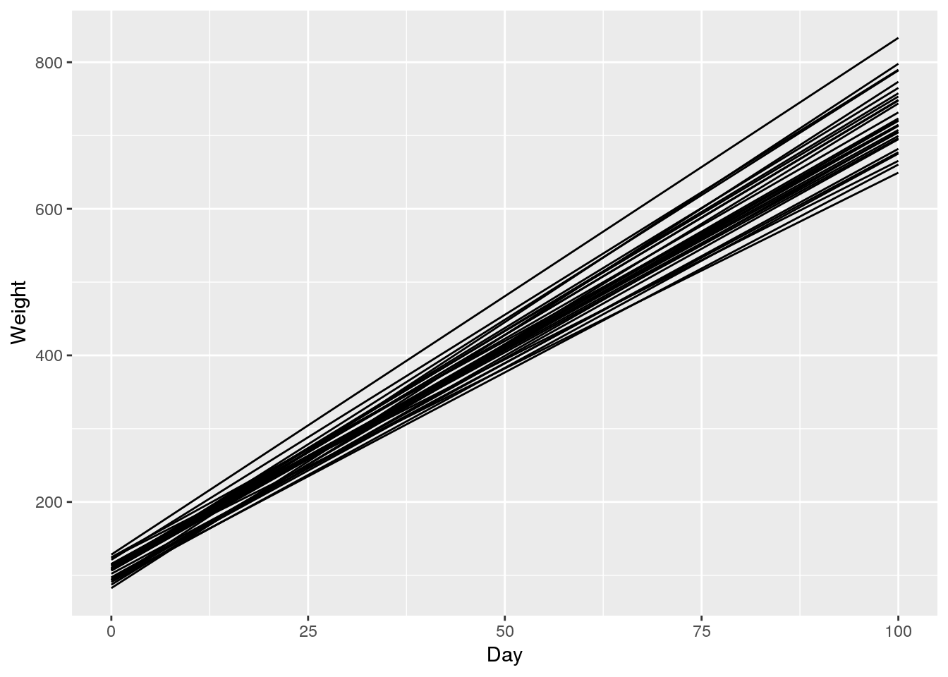
# predictions for selected rats
sel.rats <- c(9, 8, 29)
ggplot(pred.df[pred.df$Rat %in% sel.rats, ],
       aes(x = Day, y = Weight, group = Rat,
           ymin = Lwr_Weight, ymax = Upr_Weight)) +
    geom_line()  +
    geom_errorbar(width=0.2, size=0.5, color="blue")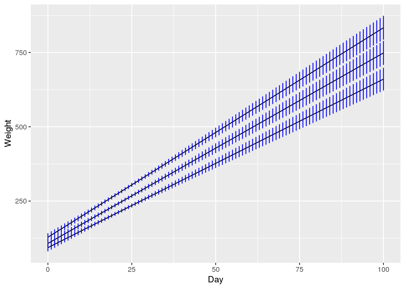
In contrast to the original data, the estimates from the model are smooth because each curve follows a linear model. Investigating the confidence intervals shown in the last plot, we can see that the variance estimates are reasonable. We are confident about the rat weights at the time of sampling (days 8 to 36) but the uncertainty increases the further we move away from the sampled region.
Where to go from here?
I am really impressed that Bayesian approaches have become so accessible through probabilistic programming. There are dozens of Stan usage examples available at GitHub. If you would like to learn more about Bayesian models, I would recommend the book Bayesian Data Analysis from Andrew Gelman.


Comments
There aren't any comments yet. Be the first to comment!