Wilcoxon Signed Rank Test vs Paired Student's t-test
The sleep data set
Let’s consider the sleep data set. The data set contrasts the effect of two soporific drugs (aka sleeping pills) by providing the change in the number of hours slept after taking the drug compared to a baseline:
data(sleep) # load the sleep data set
print(sleep)## extra group ID
## 1 0.7 1 1
## 2 -1.6 1 2
## 3 -0.2 1 3
## 4 -1.2 1 4
## 5 -0.1 1 5
## 6 3.4 1 6
## 7 3.7 1 7
## 8 0.8 1 8
## 9 0.0 1 9
## 10 2.0 1 10
## 11 1.9 2 1
## 12 0.8 2 2
## 13 1.1 2 3
## 14 0.1 2 4
## 15 -0.1 2 5
## 16 4.4 2 6
## 17 5.5 2 7
## 18 1.6 2 8
## 19 4.6 2 9
## 20 3.4 2 10extra indicates the increase/decrease (positive/negative values) in sleep compared to the baseline measurement, group denotes the drug, and ID gives the patient ID. To make this clearer, I’ll rename group to drug:
colnames(sleep)[which(colnames(sleep) == "group")] <- "drug"Note that the sleep data set contains two measurements for every patient. Thus, it is appropriate for showcasing paired tests such as the ones we are dealing with.
What are we testing for?
Assume we are working in a pharmaceutical company and these are the data that were just obtained from a clinical trial. Now, we must decide which of the two drugs you should go forward with for market release. A reasonable way of selecting the drug would be to identify the drug that performs better. More specifically, the question is the following: is one of the drugs associated with greater values of extra than the other drug?
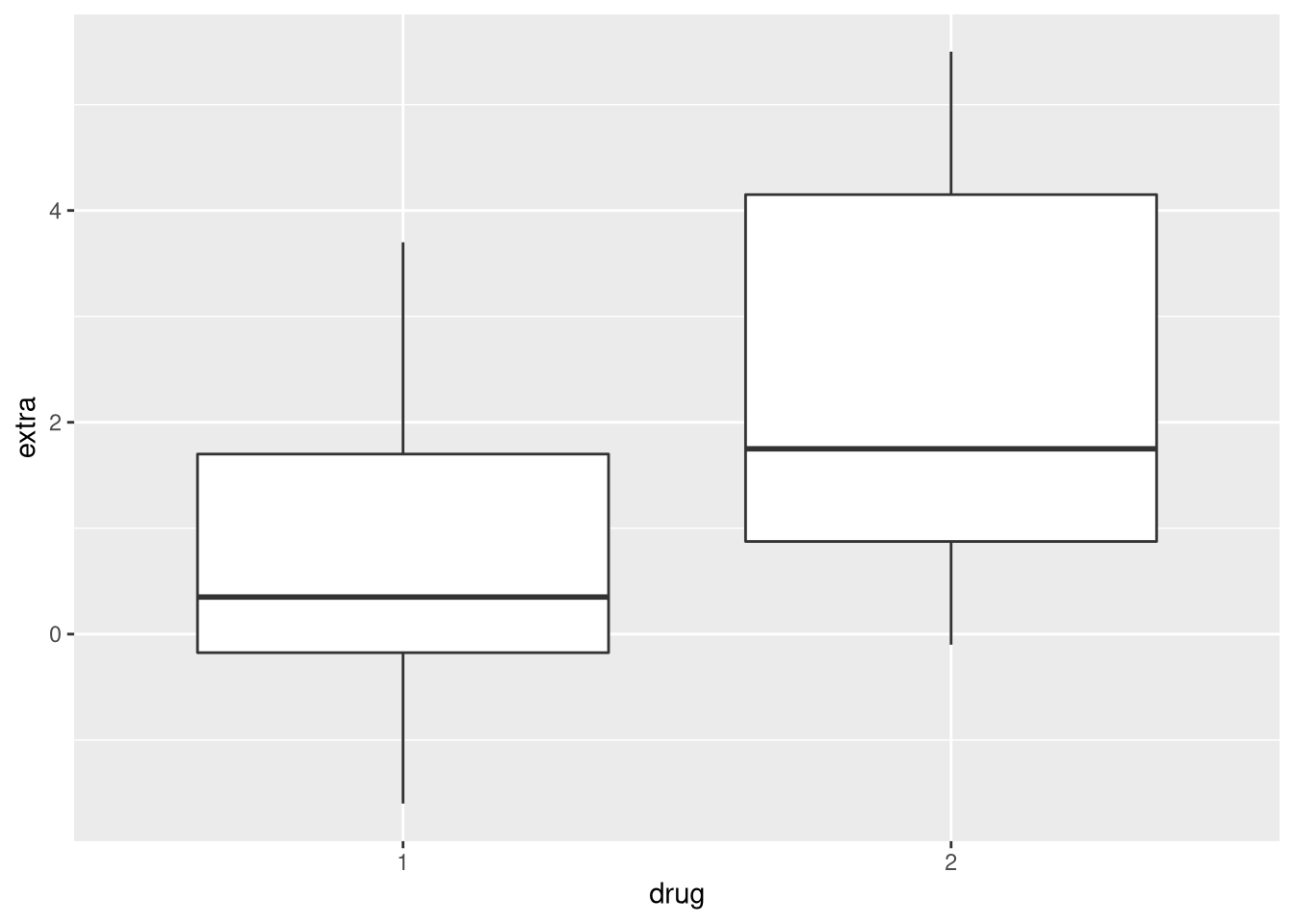
To get an intuition about the effectiveness of the two drugs, let’s plot their corresponding values:

The plot shows that the median increase in sleep time of drug 1 is close to 0, while the median increase for drug 2 is close to 2 hours. So, based on these data it seems that drug 2 is more effective than drug 1. However, we still need to determine whether our finding is statistically significant.
The null hypothesis
The null hypothesis of the test is that there isn’t any difference in the extra sleep time between the two drugs. Since we want to find out whether drug 2 outperforms drug 1, we do not need a two-tailed test (testing whether any of the drugs has superior performance), but a one-tailed test. Thus, the alternative of the null hypothesis is that drug 2 is associated with greater values of extra than drug 1.
Wilcoxon Signed Rank Test
The Wilcoxon signed rank test uses the sum of the signed ranks as the test statistic W:
W=N∑i=1[sgn(x2,i−x1,i)⋅Ri]
To perform the test in R, we can use the wilcox.test function. However, we have to explicitly set the paired argument to indicate that we are dealing with matched observations. To specify the one-tailed test, we set the alternative argument to greater. In this way, the alternative of the test is whether drug 2 is associated with larger increases in sleep duration than drug 1.
x <- sleep$extra[sleep$drug == 2]
y <- sleep$extra[sleep$drug == 1]
res <- wilcox.test(x, y, paired = TRUE,
alternative = "greater")## Warning in wilcox.test.default(x, y, paired = TRUE, alternative = "greater"):
## cannot compute exact p-value with ties## Warning in wilcox.test.default(x, y, paired = TRUE, alternative = "greater"):
## cannot compute exact p-value with zeroesInvestigating the warnings
Before getting to the results, we should investigate the two warnings that resulted from performing the test.
Warning 1: ties
The first warning arises because the test ranks differences in the extra values of pairs. If two pairs share the same difference, ties arise during ranking. We can verify this by computing the difference between the pairs
x - y## [1] 1.2 2.4 1.3 1.3 0.0 1.0 1.8 0.8 4.6 1.4and finding that pairs 3 and 4 both share the same difference of 1.3. Why are ties a problem? The rank assigned to ties is based on the average of the ranks they span. Thus, if there are many ties, this reduces the expressiveness of the test statistic rendering the Wilcoxon test inappropriate. Since we only have a single tie here, this is not a problem.
Warning 2: zero values
The second warning relates to pairs where the difference is 0. In the sleep data set, this is the case for the pair from the 5th patient (see above). Why are zeros a problem? Remember that the null hypothesis is that the differences of the pairs are centered around 0. However, observing differences where the value is exactly 0 do not give us any information for the rejection of the null. Therefore, these pairs are discarded when computing the test statistic. If this is the case for many of the pairs, the statistical power of the test would drop considerably. Again, this is not a problem for us as only a single zero value is present.
Investigating the results
The main result of the test, is its p-value, which can be obtained via:
res$p.value## [1] 0.004545349Since the p-value is less than the 5% significance level, this means we can reject the null hypothesis. Thus, we would be inclined to accept the alternative hypothesis, which states that drug 2 outperforms drug 1.
Paired Student’s t-test
The paired Student’s t-test is a parametric test on the means of paired quantitative measurements from two groups. Here, parametric means that the t-test assumes that the mean difference between samples is normally distributed. The test relies on identifying whether the mean difference of measurements from the two groups, ˉXD is larger than μD, where μD is typically set to 0 in order to find if there is any difference. The test-statistic,
t=ˉXD−μ0sD√n,
is normalized using the standard deviation of differences, sD, and the number of pairs n. By normalizing according to sD√n, the test statistic regulates the value of the test statistic according to the number of samples (|t| increases with more samples) and the standard deviation of differences (|t| decreases if the deviation increases).
In R, we can perform the paired t-test with the t.test function. Note that t.test assumes that population variances are inequal. In this case, the test is also called Welch’s t-test. To obtain the original t-test, which assumes that the population variances are equal, we can just set the equal.var parameter to TRUE. Here, we will just use with the default setting:
t.result <- t.test(x,y, paired = TRUE, alternative = "greater")
print(t.result$p.value)
## [1] 0.001416445Again, the p-value is less than 0.05. Thus, we would be inclined to accept the alternative hypothesis: drug 2 is associated with a greater increase in mean sleep duration than drug 1.
Checking the assumptions of Student’s t-test
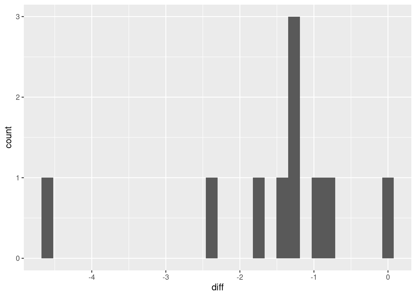
The t-test requires that the sample means are normally distributed. By the central limit theorem, means of samples from a population approach a normal distribution for a sufficient number of samples. Therefore, the assumption of the t-test is met even for non-normal measurements as long as there are is a sufficient number of samples. Since the sleep data contains only 10 paired measurements, there should be reason for concern. Thus, we should check whether the diffeerences between measurements are normally distributed in order to verify whether the t-test is valid:
diff.df <- data.frame(diff = sleep$extra[sleep$drug == 1] - sleep$extra[sleep$drug == 2])
ggplot(diff.df, aes(x = diff)) + geom_histogram()
## `stat_bin()` using `bins = 30`. Pick better value with `binwidth`.
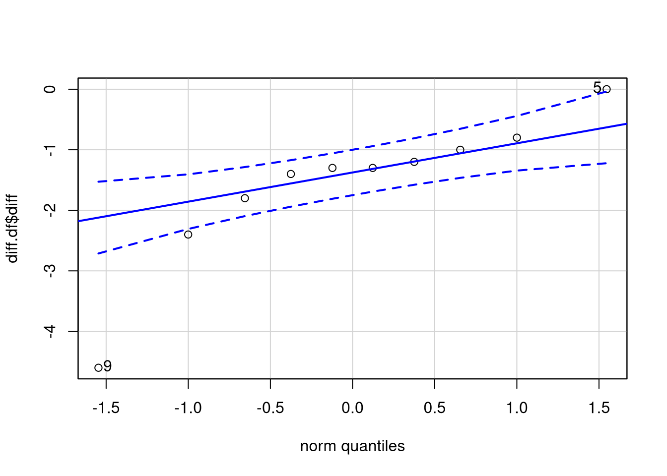
Looking at the histogram, the data seem rather uniformly than normally distributed. To take a closer look, we compare the differences to the values that would be expected from a normal distribution using a Q-Q (quantile-quantile) plot:
require(car) # load car package to use 'qqp' rather than native 'qqplot' function## Loading required package: car## Loading required package: carDataqqp(diff.df$diff)
## [1] 9 5The Q-Q plot shows that the differences fit the normal model quite well, except for the heavy tails. From this, we could conclude that the assumption of the t-test is sufficiently met. Still, we’re left with a feeling of uncertainty about whether the t-test was the most appropriate choice for these data.
Summary: Wilcoxon signed rank test vs paired Student’s t-test
In this analysis, both Wilcoxon signed rank test and paired Student’s t-test led to the rejection of the null hypothesis. In general, however, which test is more appropriate? The answer is, it depends on several criteria:
- Hypothesis: Student’s t-test is a test comparing means, while Wilcoxon’s tests the ordering of the data. For example, if you are analyzing data with many outliers such as individual wealth (where few billionaires can greatly influence the result), Wilcoxon’s test may be more appropriate.
- Interpretation: Although confidence intervals can also be computed for Wilcoxon’s test, it may seem more natural to argue about the confidence interval of the mean in the t-test than the pseudomedian for Wilcoxon’s test.
- Fulfillment of assumptions: The assumptions of Student’s t-test may not be met for small sample sizes. In this case, it is often safer to select a non-parametric test. However, if the assumptions of the t-test are met, it has greater statistical power than Wilcoxon’s test.
Due to the small sample size of the sleep data set, I’d prefer the test from Wilcoxon for these data.
Which test would you use? In general, would you prefer one test over the other?


Comments
al
17 Dec 19 10:24 UTC
The assumptions of Student’s t-test may not be met for small sample sizes. In this case, it is often safer to select a parametric test. However, if the assumptions of the t-test are met, it has greater statistical power than Wilcoxon’s test.
don’ you wanna say non parametric